Anna Go - Restricted Boltzmann Machines

Info

These notes are meant to serve as a practical tutorial providing the minimum sufficient knowledge required to build and train a Restricted Boltzmann Machine (RBM).

Introduction

In the early days of Machine Learning (ML), RBMs used to be among the top methods for the unsupervised setting, where the training data are inputs without labels and the task is, broadly speaking, to extract some meaningful information from this data.

An RBM is a parametrized generative model representing a probability distribution. The training data is assumed to be a sample drawn independently from an unknown target distribution $q$. The goal of training is to fit the parameters $\lambda$ of the RBM’s distribution $p_{\lambda}$ such that it resembles the target distribution $q$ as accurately as possible.

Formally, RBMs belong to the class of undirected graphical models, also known as Markov Random Fields (MRFs). Probabilistic graphical models describe probability distributions by mapping conditional (in)dependence properties between random variables on a graph structure. Visualization by graphs is useful for understanding and motivating probabilistic models. Moreover, it can be helpful for deriving complex computations by using algorithms that exploit the graph structure. Much can be said about the theoretical properties of graphical models and the implications for RBMs. However, with the goal of keeping this tutorial short and hands-on, I omit this discussion here and refer to the references provided at the end.

RBM definition

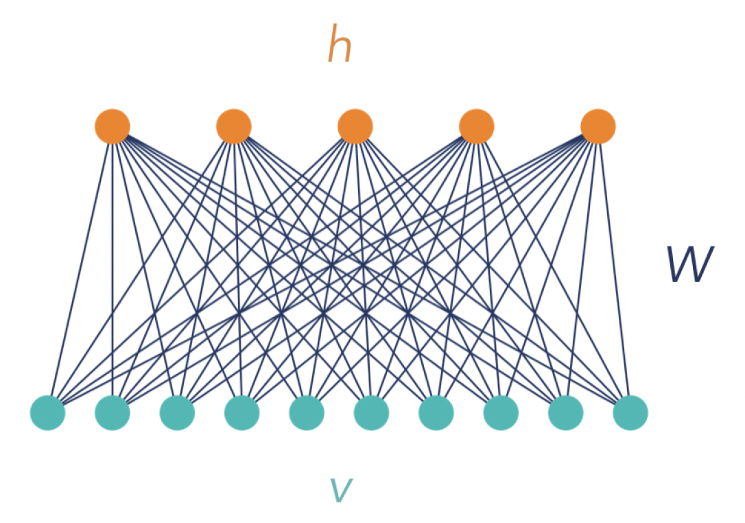
Practically, an RBM is a single-layer network with bidirectionally connected stochastic processing units, as shown in Figure 1. Units denoted by the vector $v=(v_1, ..., v_V)$ correspond to the components of an observation (input) and are therefore called “visible”, while the $H$ units on the top, denoted $h=(h_1, ..., h_H)$, represent latent variables, and are referred to as “hidden”. Hidden units model dependencies between the observation components and can be viewed as feature detectors. The term “restricted” refers to the connections between the units: Each visible unit is connected with each hidden unit, but there are no connections between units of the same kind. In the simplest case (which is the case considered in this tutorial), all units are binary, such that $v \in \mathcal{V} = \{0,1\}^V$ and $h\in \mathcal{H} = \{0,1\}^H$, where curved letters $\mathcal{V}$ and $\mathcal{H}$ are used to denote the space of the visible and hidden vectors, respectively. Further, we denote the training set containing $m$ input instances (observations) as $\mathcal{S}_m$.

Figure 1: RBM as a bipartite graph with hidden units $h$, visible units $v$ and connecting weights $W$.

In analogy to spin models in statistical physics, the joint configuration $(v,h)$ of visible and hidden units is characterized by an energy: \[\begin{align} E_{\lambda}(v,h) &= - a^\top v - b^\top h -h^\top Wv \\ \nonumber &= - \sum\limits_{i=1}^V a_i v_i - \sum\limits_{j=1}^H b_j h_j - \sum\limits_{ij} v_i W_{ij} h_j, \end{align}\] where $v_i, h_j$ are binary states of the visible unit $i$ and the hidden unit $j$, and $a_i$, $b_j$ are their respective biases. $W_{ij}$ is the symmetric connection weight between the units. The complete set of parameters is denoted by $\lambda = \{a,b,W\}$. All parameter values are real numbers.

Based on this energy function, the RBM assigns a probability to each joint configuration $(v,h)$, which by convention is high when the energy of the configuration is low: \[ p_{\lambda}(v,h) = \frac{1}{Z} e^{-E_{\lambda}(v,h)} \tag{1}\] known as the Gibbs distribution. The partition function $Z$ is given by summing over all possible pairs of visible and hidden vectors: \[ Z = \sum\limits_{v\in \mathcal{V}}\sum\limits_{h\in \mathcal{H}} e^{-E_{\lambda}(v,h)} \]

What we actually want to model is the probability distribution of an input vector $v$, $p_{\lambda}(v)$. It is obtained by marginalizing the joint probability distribution $p_{\lambda}(v,h)$ over all possible hidden vectors $h$: \[\begin{equation} p_{\lambda}(v) = \frac{1}{Z} \sum\limits_{h\in \mathcal{H}} e^{-E_{\lambda}(v,h)}. \end{equation}\] By carrying out the sum over $h$, one obtains a related expression: \[\begin{equation} p_{\lambda}(v) = \frac{1}{Z} e^{-\mathcal{E}_{\lambda}(v)} \end{equation}\] where $\mathcal{E}_{\lambda}(v)$ is the effective energy, defined as \[\begin{align*} \mathcal{E}_{\lambda}(v) &= -a^\top v - \sum\limits_{j=1}^H \ln\left[ 1 + \exp(b_j + \sum\limits_{i} W_{ij}v_i) \right]\\ &= -a^\top v - \sum\limits_{j=1}^H \text{softplus}\left(b_j + \sum\limits_{i} W_{ij}v_i\right) \end{align*}\]

Training

Training the RBM means adjusting parameters $\lambda$ based on the given data set $\mathcal{S}_m$, such that $p_{\lambda}(v)$ is a good approximation of $q(v)$. However, unlike in the supervised setting where we have access to the target labels, here the target distribution $q$ is unknown. All we have available is the set of $m$ samples drawn from $q$; therefore, we will have to make approximations to compute terms involving $q$.

There are two ways of formulating the training objective for RBMs: One uses the Kullback-Leibler (KL) divergence as the loss function to minimize, while the other relies on the Maximum-Likelihood method. Both of these methods lead to the same equations, as we shall see below.

KL divergence as a loss function

The KL divergence is a measure for discrepancy between the learned and the target probability distribution, defined as follows: \[ D_{KL}(q\| p_{\lambda}) = \sum\limits_{v} q(v) \ln \frac{q(v)}{p_{\lambda}(v)} = - [H(q) + \langle \ln p_{\lambda}(v) \rangle_{q}] \tag{2}\] Using KL as the loss function, the training objective is to minimize KL via gradient descent. However, note that in Equation 2, the term $H(q)$—the Shannon entropy of the target distribution—is independent of the parameters $\lambda$ and therefore irrelevant for the optimization. What remains as the loss function is the expectation value of the negative log-likelihood: \[ \text{Loss} = - \langle \ln p_{\lambda}(v) \rangle_{q} = - \sum\limits_{v} q(v) \ln p_{\lambda}(v) \] Therefore, minimizing the KL divergence is equivalent to maximizing the log-likelihood. The following section shows how one arrives at an equivalent training objective via the maximum-likelihood method without defining the KL divergence as a loss function.

The maximum-likelihood method

Consider that the number of all theoretically possible visible vectors is $|\mathcal{V}| = 2^V$, but only a small number from the entire set are actually existent configurations, and a subset of these is contained in the training set. Therefore, we can assume that the probability of those configurations which we observe in the training set is high. Thus, the training goal is to make $p_{\lambda}(v)$ large for all $v$ from the training set $\mathcal{S}_m$, and small for the other $v\notin \mathcal{S}_m$. In other words, we want to find parameters $\lambda$ that maximize the probability of $\mathcal{S}_m$ under the distribution $p_{\lambda}$. The outlined approach is the standard way of estimating the parameters of a statistical model, called maximum-likelihood estimation (MLE).

The maximum-likelihood method is based on the likelihood function $\mathcal{L}(\lambda | \mathcal{S}_m )$, which describes the likelihood of the parameters $\lambda$ given the data $\mathcal{S}_m$, and is defined as \[ \mathcal{L}(\lambda | \mathcal{S}_m ) = \prod\limits_{v\in \mathcal{S}_m} p(v | \lambda), \] where $p(v | \lambda) = p_{\lambda}(v)$.

The goal is to find the set of parameters $\lambda$ that maximizes the likelihood. In practice, it is more convenient to work with the natural logarithm of the likelihood function, called the log-likelihood: \[ \ell (\lambda | \mathcal{S}_m ) \equiv \ln \mathcal{L}(\lambda | \mathcal{S}_m ) = \sum\limits_{v\in \mathcal{S}_m} \ln p_{\lambda}(v). \] This is the objective function of the unsupervised learning procedure.

An aside: “Likelihood” and the basics of inference

Likelihood is a term from Bayesian inference – a technique in statistical inference based on the Bayes’ theorem. Statistical inference is the process of using data analysis to deduce properties of the underlying probability distribution. Bayes’ theorem is used to update the probability for a hypothesis as more evidence (i.e., information related to the hypothesis) becomes available. Mathematically, it can be stated as follows: \[ P(H | E, \lambda) = \frac{ P(E | H, \lambda) P(H) }{ P(E | \lambda) }, \] where $H$ corresponds to the hypothesis, $E$ to the evidence, and $\lambda$ denotes the parameters that affect the evidence.

Now, the terminology:

The marginal probability $P(H)$ is the prior probability of $H$.
$P(E | H, \lambda)$ is the likelihood of $H$.

It is important to note that the terms “probability” and “likelihood” are not interchangeable. $P(E | H, \lambda)$ is a function of both $E$ and $H$: For fixed $H$, it defines a probability over $E$, and for fixed $E$, it defines the likelihood of $H$. The likelihood function is not a probability distribution!
$P(H | E, \lambda)$ is the posterior probability of $H$ given $E$.
The normalizing constant $P(E | \lambda)$ is the marginal likelihood, also called “evidence”.

In words, the core of Bayesian inference can be summed up as follows: \[ \text{posterior} = \frac{ \text{likelihood $\times$ prior} }{ \text{evidence} } \]

Gradient Descent on the Negative Log-Likelihood

We minimize the negative log-likelihood by performing gradient descent. The update rule for the weight (and analogously for the biases) takes on the following familiar form: \[ W \leftarrow W - \eta \nabla_W (- \ell(\lambda | v)), \] where $v\in \mathcal{S}_m$, $\eta$ is the learning rate, and we have assumed online learning, i.e., the update is performed for each training example.

To compute this, we require the derivative of the log-probability of a visible vector with respect to a weight, which turns out to be very simple: \[ \frac{\partial\ln p_{\lambda}(v) }{\partial W_{ij} } = \left\langle v_i h_j \right\rangle_{\text{data}} - \left\langle v_i h_j \right\rangle_{\text{model}} \tag{3}\] where the angled brackets denote expectation values under the distributions specified by the subscript; explicitly: \[ \langle v_i h_j \rangle_{\text{data}} = \sum\limits_{h} v_i h_j p_{\lambda}(h|v), \tag{4}\] \[ \langle v_i h_j \rangle_{\text{model}} = \sum\limits_{v,h} v_i h_j p_{\lambda}(v,h). \tag{5}\]

Derivation

Here is an explicit derivation of the above result.

\[\begin{align} \frac{\partial \log p(v) }{\partial W_{ij} } &= \frac{ \partial }{\partial W_{ij} } \log\left[ \frac{1}{Z} \sum\limits_{h} e^{-E(v,h)} \right]\\ &= \frac{\partial }{\partial W_{ij} } \left\{ \log \left[ \sum\limits_{h} e^{-E(v,h)} \right] - \log Z \right\}\\ &= \left[ \sum\limits_{h} e^{-E(v,h)} \right]^{-1} \frac{\partial }{\partial W_{ij} } \sum\limits_{h} e^{-E(v,h)} - Z^{-1} \frac{\partial }{\partial W_{ij} } Z \\ &= \left[ Z p(v) \right]^{-1} \frac{\partial }{\partial W_{ij} } \sum\limits_{h} e^{-E(v,h)} - Z^{-1} \frac{\partial }{\partial W_{ij} } Z \\ &= \left[ Z p(v) \right]^{-1} \sum\limits_{h} v_i h_j e^{-E(v,h)} - Z^{-1} \sum\limits_{v,h} v_i h_j e^{-E(v,h)} \\ &= \sum\limits_{h} v_i h_j \frac{p(v,h)}{p(v)} - \sum\limits_{v,h} v_i h_j p(v,h) \\ &= \sum\limits_{h} v_i h_j p(h|v) - \sum\limits_{v,h} v_i h_j p(v,h) \end{align}\]

\[\begin{align} \frac{\partial }{\partial W_{ij} } \sum\limits_{h} e^{-E(v,h)} &= \frac{\partial }{\partial W_{ij} } \sum\limits_{h} \exp\left[ \sum\limits_{k} a_k v_k + \sum\limits_{l} b_l h_l + \sum\limits_{kl} v_k W_{kl} h_l \right] \\ &= e^{a^\top v} \sum\limits_{h} e^{b^\top h} \frac{\partial \exp\left[ \sum\limits_{l} b_l h_l \right] }{\partial W_{ij} } \\ &= e^{a^\top v} \sum\limits_{h} e^{b^\top h} v_i h_j e^{v^\top W h} \\ &= \sum\limits_{h} v_i h_j e^{-E(v,h)} \end{align}\]

\[\begin{align} \frac{\partial }{\partial W_{ij} } Z &= \frac{\partial }{\partial W_{ij} } \sum\limits_{v,h} e^{-E(v,h)} \\ &= \sum\limits_{v} \frac{\partial }{\partial W_{ij} } \sum\limits_{h} e^{-E(v,h)} \\ &= \sum\limits_{v,h} v_i h_j e^{-E(v,h)} \end{align}\]

Because there are no direct connections between units of the same layer in an RBM, the conditional probabilities $p_{\lambda}(h|v)$ and $p_{\lambda}(v|h)$ factorize and are easy to compute. With some straightforward algebra, one can show that \[ p_{\lambda}(h | v) = \prod\limits_{j} p_{\lambda}(h_j | v) \tag{6}\] \[ p_{\lambda}(v | h) = \prod\limits_{i} p_{\lambda}(v_i | h) \tag{7}\] and \[ p_{\lambda}(h_j=1 | v) = \sigma\left( b_j + \sum_i v_i W_{ij} \right) \tag{8}\] \[ p_{\lambda}(v_i=1 | h) = \sigma\left( a_i + \sum_j h_j W_{ij} \right) \tag{9}\] with $\sigma$ denoting the standard logistic sigmoid function: \[ \sigma(x) = \frac{1}{1+e^{-x}}. \] The expectation value $\langle v_i h_j \rangle_{\text{data}}$ in Equation 4 can be simplified by explicitly carrying out the sum over $h$ and using Equation 6: \[ \langle v_i h_j \rangle_{\text{data}} = v_i \sum\limits_{h_1\in\{0,1\}} \dots \sum\limits_{h_H\in\{0,1\}} h_j \prod\limits_{j'=1}^H p_{\lambda}(h_{j'} | v) = v_i~p_{\lambda}(h_j=1 | v). \] Note that \[\begin{equation} \frac{\partial E_{\lambda}(v,h) }{\partial W_{ij} } = -v_i h_j \end{equation}\] can be written in matrix form as \[ \nabla_W E_{\lambda}(v,h) = -h v^\top, \tag{10}\] where $h$ is a column vector and $v^\top$ is a row vector (i.e., this is an outer product between the hidden and the visible vector). Then, the weight update rule takes on the following form: \[\begin{align} W &\leftarrow W - \eta \left( \left\langle \nabla_W E_{\lambda}(v,h) \right\rangle_{\text{data}} - \left\langle \nabla_W E_{\lambda}(v,h) \right\rangle_{\text{model}} \right)\\ W &\leftarrow W - \eta \left( \sum\limits_{h} p_{\lambda}(h|v) \nabla_W E_{\lambda}(v,h) - \sum\limits_{v,h} p_{\lambda}(v,h) \nabla_W E_{\lambda}(v,h) \right). \end{align}\] Using Equation 10, Equation 4, Equation 6, Equation 8, the first expectation can be written as \[ \left\langle \nabla_W E_{\lambda}(v,h) \right\rangle_{\text{data}} = - \left\langle h v^\top \right\rangle_{\text{data}} = -\sigma\left( b + Wv \right) v^\top \tag{11}\] – neat and readily computable.

The term $\left\langle \nabla_W E_{\lambda}(v,h) \right\rangle_{\text{model}}$, however, poses a serious challenge. This expectation value is over the joint probability distribution $p_{\lambda}(v,h) = e^{-E_{\lambda}(v,h)}/Z$ and involves the partition function $Z$ (which conveniently cancelled out in the expressions for the conditional probabilities). $Z$ requires evaluation of the sum over all $h\in\mathcal{H}$ and $v\in\mathcal{V}$, and is thus in general intractable. There are several possible approximate methods to handle this term, but not all of them are practicable. A straighforward approach is to approximate the expectation $\left\langle \cdot \right\rangle_{\text{model}}$ by sampling from the model distribution using Gibbs sampling.

Gibbs Sampling

In Gibbs sampling, each variable is sampled from its conditional distribution given the current states of the other variables. A randomly initialized state is used as the starting point. In RBMs, this procedure is particularly efficient because the visible units are conditionally independent given the hidden units (and vice versa), such that the calculation can be carried out for all hidden units in parallel, as illustrated in Figure 2. This is referred to as Block Gibbs Sampling. However, to ensure that the Markov chain converges to stationarity, the sampling process has to be run for a long time. Since this step has to be repeated for each parameter update in the learning procedure, this technique is computationally not feasible. Therefore, all methods that are employed in practice introduce additional approximations.

Contrastive Divergence

The standard learning algorithm employed for RBM training is called Contrastive Divergence (CD-$k$, where $k$ indicates the number of iterations). Essentially, the idea of this algorithm is to perform only $k$ steps of Gibbs sampling, starting from a current training vector $v=v^{(0)}$. Then the expectation $\langle \cdot \rangle_{\text{model}}$ is replaced by a point estimate $\langle \cdot \rangle_{\text{reconstr}}$ computed at $\tilde{v}=v^{(k)}$. Even though it is only crudely approximating the true expectation, learning works surprisingly well. In general, larger $k$ yields a less biased estimate; however, $k=1$ is often sufficient to extract meaningful features in practice.

The main steps of the CD-$k$ learning procedure are:

Start by setting the visibles to a training vector $v$.
Perform the following Gibbs sampling procedure $k$ times:
- Compute the states of the hiddens (in parallel) by setting each unit to 1 with a probability given by Equation 8.
- Produce a “reconstruction” of $v$ (denoted as $v^{(i)}$, where $i$ is the iteration step number), by setting each visible to 1 with a probability given by Equation 7.
Use $\tilde{v} = v^{(k)}$ to compute the point estimate $\langle \cdot \rangle_{\text{reconstr}}$ and update the parameters.
Go back to step 1 and repeat the procedure until all stopping criteria are fulfilled.

Thus, in this approach, the expectation value \[ \sum\limits_{v,h} p_{\lambda}(v,h) \nabla_W E_{\lambda}(v,h) \] is replaced by \[ \sum\limits_{h} p_{\lambda}(h | \tilde{v}) \nabla_W E_{\lambda}(\tilde{v},h). \] Using Equation 11, the CD update rule for the weights can be written as follows: \[ W \leftarrow W + \eta \left[ \sigma\left( b + Wv \right) v^\top - \sigma\left( b + W\tilde{v} \right) \tilde{v}^\top \right], \] with a training example $v\in \mathcal{S}_m$ and the so-called “negative sample” $\tilde{v}$, obtained from $v$ by Gibbs sampling.

A simplified version of the same learning rule is applied to the biases; it involves the states of individual units instead of pairwise products: \[ a \leftarrow a + \eta \left( v-\tilde{v} \right), \] and \[ b \leftarrow b + \eta \left[ \sigma\left( b + Wv \right)-\sigma\left( b + W\tilde{v} \right) \right]. \] Note that some references define a short-hand notation $\sigma\left( b + Wv \right) \equiv h(v)$, because the logistic function essentially defines the state of $h$. However, it is important to keep in mind that $h$ is a binary vector, and $\sigma\left( b + Wv \right)$ does not provide the values, but the {} for each element of $h$ having the value 1. This actually leads to the following practical remark:

Computing the state of a binary unit

Given a visible vector $v$ and the set of parameters $\lambda$, how do we compute the state of a hidden unit $h_j$? Since the unit is binary, its state is sampled according to the Bernoulli distribution with the probability for $h_j$ having the value 1 given by Equation 8. In practice, we sample a number $u$ from a uniform distribution over the interval $[0,1]$, $u\sim U[0,1]$. If $u < p_{\lambda}(h_j = 1 | v)$, set $h_j=1$, otherwise $h_j=0$.

Persistent Contrastive Divergence

A slight modification of the CD algorithm leads to the Persistent Contrastive Divergence (PCD) algorithm~. In PCD, instead of initializing the chain to $v^{(0)} = v \in\mathcal{S}_m$ each time, we use the negative sample from the previous iteration, $v^{(0)} = \tilde{v}$. That is, PCD just keeps the Markov chain evolving, with parameter updates done after each $k$ steps. The number of persistent chains used for sampling is a hyperparameter. In the standard case, there is one Markov chain per training example in a batch.